MATLAB transform fundamentals

Analyzer 2 in practice: MATLAB® transform fundamentals

by Patrick Britz, Sales

When you open the MATLAB® transform, you see only a single, uncluttered dialog box. But don’t get misled by this Spartan look: It’s a very powerful tool that combines the advantages of two different worlds and allows you to access numerous functions. Approaching the challenge slowly, we’ll begin with an introduction to the dialog box. Then you’ll learn some useful little tricks, and we’ll finish off with a little MATLAB® code that allows you to explore your data with a t-test. Clearly, most of what we are doing here we can also do in Analyzer 2.0. But the point of
this is to provide a demonstration of the Matlab interface.

To display the transform dialog box, choose Transformations > Others > Matlab. The dialog box is shown in Figure 1. The first thing you have to do is to decide whether you want to have the calculation done on request or when a node is created (by selecting the corresponding radio button). After we have gone through the examples below, it will be clear to you which option you need to choose when. Two of the check boxes shown are only required if you want to work in EEGLAB or with EEGLAB functions. You can either export your EEG to MATLAB® in EEGLAB format or you can additionally have EEGLAB start up immediately after the data is transferred by clicking the second option as well. The other three check boxes allow you to adjust performance. They
are of course described in the manual.

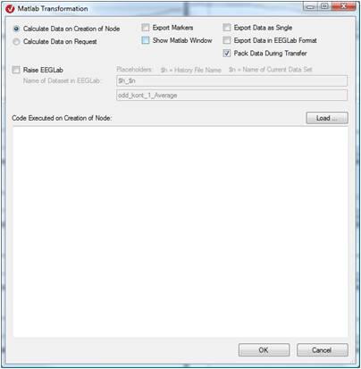
Figure 1

If you select the “Calculate Data on Request” radio button, a second text box appears in the dialog box. In this text box you can enter the MATLAB® code to be processed on request. The dialog box will be as shown in Figure 2.

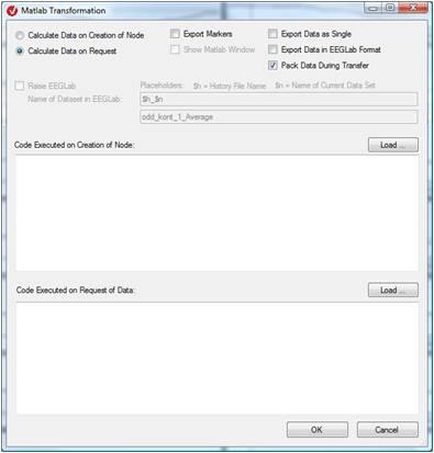
Figure 2

The first text box works in the same way in both cases. You can enter all the code required to process your EEG data, set properties and create new markers in the “Code Executed on Creation of Node” text box.

You need to know the fundamentals of MATLAB® to gain full benefit from this tool. If you are not already an expert MATLAB® user, it will help if you go through the MATLAB® “Getting started” manual.

First example – rearranging the channels

In order to check that all ocular artifacts have been removed from the data after ocular correction, you generally compare the frontal channels with the ocular channels. In other words, you compare HEOG and VEOG with the channels FP1, FPZ and FP2. Unfortunately, in the standard view the FP1, FPZ and FP2 channels are generally right at the top and the VEOG und HEOG channels are at the bottom of the list. It would be nice to have these channels next to each other in order to compare them.

For a data set with 32 channels, the next two lines of code put the last two channels in the first two positions, followed by the remaining channels. The first line rearranges the lines of the data matrix (i.e. the data), while the second line rearranges the descriptions of the channels accordingly (i.e. the names and coordinates).

EEGData = EEGData(:,[31 32 1:30]); Properties.Channels = Properties.Channels(:,[31 32 1:30]);

To try it out, simply copy these two lines of code to the “Code Executed on Creation of Node” text box and click “OK”. You get a node called “Matlab transform” that contains the channels rearranged in the new order. Aren’t you already just a little bit impressed by how easy it is to use Matlab in Analyzer 2.0? You don’t have to worry about importing or exporting. That all takes place fully automatically in the background, and this node is, of course, template-capable.

Second example: “Calculate Data on Request” option

So what do we need the “Calculate Data on Request” option for? Well, when this radio button is selected, the transform is always applied to that portion of the data that is currently displayed. It is therefore ideal for creating additional views of the data.

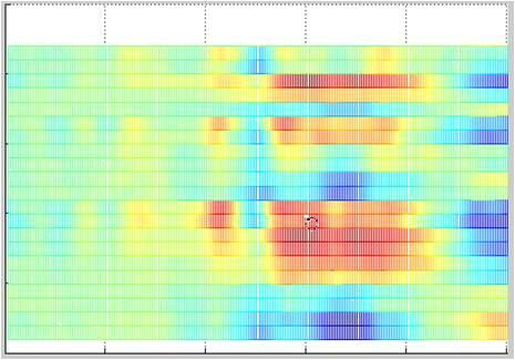
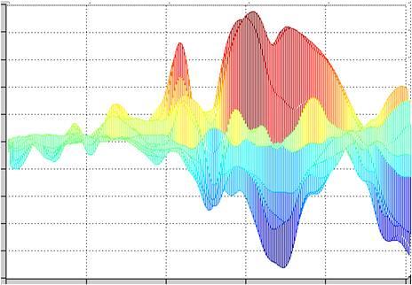
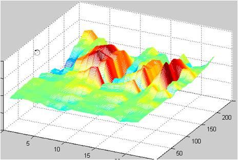
Matlab offers a wide range of data visualization options. Figure 3 shows three options that can be helpful for data visualization. In all three plots, the amplitude values are color-coded. Plot 3a shows an EEG in the form of color-coded values. The channels are arranged along the y-axis, and the data points are shown along the x-axis (i.e. time multiplied by sampling rate). Plot 3b shows the channels as curves one behind the other, and plot 3c shows a waterfall plot.

Figure 3a, 3b & 3c

So how many pages of code do we need to write to get the three plots shown in Figure 3? In fact, we need only the three lines of Matlab code shown below. These display the current data matrix “EEGData” with the Matlab plot “mesh”. The “mesh” plot can be rotated using the relevant tool in Matlab. The three plots in Figure 3 thus show exactly the same data and the same plot, but in each case from a different point of view. Not bad, eh?

[AZ,EL] = view;
mesh(EEGData);
view(AZ, EL);

After the transform is executed or when the node is opened again, the Analyzer initially shows the first 10 seconds of data. This is exactly the data we see in the Matlab graphic.

To find out what the “Calculate Data on Request” option does, select a section of your data and click the “Zoom in” button on the Analyzer 2.0 toolbar or navigate along your data. The Matlab plot always shows exactly the data that you can currently see in the Analyzer.

Third example: t-test

Now it’s time to move on to a more complex example. We’ll take a small fictitious data set as an example. Then we’ll go through the steps required to explore a data set like this in Matlab using a t-test. To do this, you have to write all of the data to a file and then load this file in Matlab. The matrix you get by loading the file has to be put into a useful form. The t-test is then calculated.

Let’s assume we have carried out a simple experiment on five people. The experiment has a repeated measurement factor with two levels. Our sampling rate is 250 Hz. We are interested to know if there are “significant” differences at Spacio-temporal areas (e.g. electrodes and timepoints). And yes, the word “significant” is placed in quotes here deliberately.

We could calculate the difference curve between the two conditions for all electrodes and display these difference curves. Unfortunately, the difference curves don’t say anything about the associated variances or the number of observations on which the difference is based.

So we want to calculate a t-test for each point in time for each electrode. To this end, we first need to get the average-value nodes of the two conditions for each person in Matlab. The Matlab transform in Analyzer 2 transfers the data of only one node to Matlab, so we first have to aggregate the data in a single file.

This can be done in a single step, but beforehand it is advisable to set the working directory of Matlab correctly (so that we can find our data subsequently):

cd (‘D:\My_EEG‘);

Now we need a command that gets Matlab to create a file and write the data to it node by node. The line of code below writes the “EEGData” matrix to the “myEEGfile.txt” file. If the “myEEGfile.txt” does not yet exist, this command creates the file first. The “-append” parameter is important here. Without it, Matlab overwrites the file with each new node.

dlmwrite(‚myEEGfile.txt‘,EEGData, ‚delimiter‘, ‚\t‘, ...
‚precision‘, 8, ‚-append‘);

So we call the Matlab transform, copy the above code to the “Code Executed on Creation of Node” text box and click “OK”. We then add the new node after each average-value node that we want to have in our file. We do this either by dragging and dropping the node on the desired nodes or by creating a corresponding history template and then running it for our five test subjects.

There should now be a file called “myEEGfile.txt” in Matlab’s working directory. We open this file by using the appropriate Matlab dialog as follows: > File > Import Data …

After we do this, the Matlab workspace contains a matrix called “myEEGfile” that is 2500 by 32 in size. You will notice that the second dimension is the number of channels. The first dimension is the number of average-value nodes (10) multiplied by the number of data points per average-value node. In our case, there are 250 data points (a second of data at 250 Hz).

We can now take a look at this matrix in Matlab. We do this either by clicking it and then clicking “plot” or by means of the following line of code:

plot(myEEGfile, ‚DisplayName‘, ‚myEEGfile‘, ‚YDataSource‘, ‚myEEGfile‘);

All of the averages are drawn one behind the other, as shown in Figure 4.

Clearly, this plot is not ideal, however, because it continues to draw the channels from one average to the next.

Figure 4

It’s clear we need to put our data matrix into a useful form: in other words, to turn our 2D matrix of 2500 by 32 into a 3D matrix with 10 averages by 32 channels by 250 data points. The first line of the code below rearranges the original matrix (myEEGfile) column by column to form a new matrix (AllAvgs). As a result of the column-based approach, however, the dimensions of the matrix are no longer in the desired order. This is dealt with by the second line of code, which shifts the second dimension (averages) to first place, the third dimension (channels) to second place and the first dimension (sampling points) to last place.

AllAvgs = reshape(myEEGfile,[250 10 32]);
AllAvgs = permute(AllAvgs, [2 3 1]);

You can no longer display this 3D matrix by means of a 2D plot. To display the first layer (i.e. the first average) of this new matrix, you have to assign it to a new matrix. The “squeeze” command reduces the emerging 3D matrix by a single dimension to form a 2D matrix.

firstAvg = squeeze (AllAvgs(1,:,:));

We can, of course, now do this for all of our 10 averages, but it’s easier if we use the Matlab function „subplot“. This allows us to arrange the various graphs (see Figure 5). The following code shows our 10 averages in two columns containing five lines each:

for count = 1:10;
subplot(5,2,count);
Avg = squeeze (AllAvgs(count,: ,:));
plot(Avg, ‚DisplayName‘, ‚Avg‘, ‚YDataSource‘, ‚Avg‘);
end

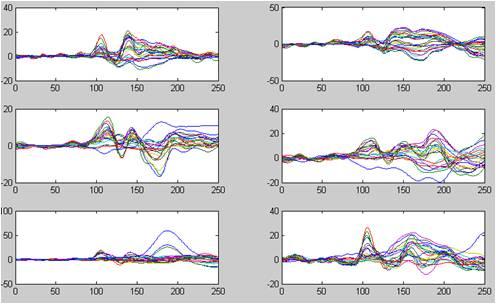
Figure 5

Incidentally, if you change the code above from “(count,: ,:)” to “(:,count, :)”, you will see an overlay of all of the averages (in our case 10) for the first 10 channels. Moreover, if you use the line “imagesc(Avg);” instead of the line “plot (Avg…)” above, you will get color-coded plots like the one in Figure 3a.

Let’s turn our attention to the t-test now. To make it easier to follow, I’ve divided it up into three steps, but you can, of course, put everything in a single line. We begin by arranging our two conditions in the two matrices “Condition1” and “Condition2”. We then calculate a t-test of the two matrices against each other. Matlab always calculates the t-test across the first dimension of the matrices. That means we don’t have to carry out any further rearrangement here. The result of a t-test consists of two matrices in our case. The first matrix (“h”) makes a statement about the acceptance or rejection of the null hypothesis and contains only the values zero and one. Zero means the null hypothesis is accepted, and one means it is rejected. The second matrix (“pValues”) contains the p-values for the t-test. The last line displays the p-values for each channel and each point in time.

Condition1 = AllAvgs ([1 3 5 7 9 11],: ,:);
Condition2 = AllAvgs ([2 4 6 8 10 12],: ,:);
[h,pValues] = ttest(Condition1, Condition2);
imagesc(squeeze (pValues));

We have just calculated a t-test for each data point and each channel. Admittedly, that was a lot of tests so let’s not get into the subject of multiple testing just yet. Clearly, we are only exploring our data here.

But it’s a great way to do it, isn’t it? And it’s possible to do it even more elegantly than we’ve done it here. If you want, you can put all of the code in a “.m” file and run it automatically just like an Analyzer template. Alternatively, you can use EEGLab functions to display your data (or p-values) in a more EEG-like way.

Many thanks for reading this article. Until next time.