
Tip: Start typing in the input box for immediate search results from our Resources Knowledge Base.
For a more comprehensive search, use the site search in the main menu above.
Manuals & Operating Instructions | Contact Support
An introduction to the ICA
Analyzer 2 in practice: The ICA transform is as easy as a walk in the park
By Patrick Britz
In the last Press Release you heard a lot about the new Analyzer 2 with its easy-to-use interface, enhanced workflow as well as its extended capabilities. Today I will show you how this affects your daily work by taking a closer look at one of the numerous transforms in Analyzer 2.
I have chosen the ICA transform (Independent Component Analyses) for this purpose, not only because it is such a versatile and widely used method but also because it is an analyzing step in which a lot of expert knowledge is considered necessary. How do you spot an expert ICA user? Well, it would seem that an expert has the ability to tell at a glance: “This IC is clearly a myogen artifact, this IC is eye-activity and this one looks like a real EEG.”
How do you become an Expert ICA user?
This leads us to the question: how do you become an Expert ICA user? Firstly, of course, it’s important to read the relevant information and to understand the background of the methods, but most importantly, you have to get a feel for the tool. Play around with your data and possibly someone else’s. I know the word “play” can sound like something requiring no effort and the ICA transform is definitely not considered to be the easiest thing to come to grips with. In fact, it has somewhat of a reputation for being very complex and a drain on a computer’s resources – but let’s see.
Below I will tell you how to really explore your ICs using Analyzer 2. But first we should take a quick look at the idea of the ICA transform and briefly discuss setting up an ICA analysis to improve performance.
The ICA transform
The ICA transform is used to split the EEG signals up into independent components using information theory methods. It is assumed here, that EEG signals are a linear combination of independent components (independent as defined in information theory).
The purpose of the ICA transform in what is known as “blind source separation” is to reconstruct source signals from a combination of these signals. Both the source signals and the combination are unknown, so assumptions are made about the signals and how they are combined. It is assumed that the signals to be reconstructed are statistically independent of each other and accordingly, the ICA transform is a purely statistical method. It is based on the above assumptions and does not use any additional physiological information. No, it does not have any information about the channel locations nor does it know anything about head shape. Therefore, it never ceases to amaze me to see the results being so intuitively linked to physiological processes or artifacts.
The result of the ICA transform is a set of components that are defined analogously to EEG channels in the time domain. In addition, the ICA transform provides a transformation matrix by means of which the component activations can be calculated from the channel data.
A more detailed description of the method and all the parameters you can set for your ICA transform can be found in the Analyzer manual. The manual is definitely worth reading and I promise it is clear and easy to understand. You will be able to find out: Why the fast ICA is not always faster than the Infomax ICA (because the fast ICA requires data with good separability of components in order to be fast) and what’s the difference between the various options you can select while setting up your analysis (e.g. some ICA algorithms are deterministic and some are not and will therefore lead to slightly different results every time you run them). In addition the manual will guide you nicely through all the steps you need in order to set up an ICA analysis which I don’t have time or space to talk about now.
Once we’ve addressed the theoretical elements we’ll take a quick look at the steps needed to run an ICA. There is only one other thing we need to discuss before that: the data on which you want to run the ICA, because ICA results strongly depend on the quality of the data.
The data
The ICA transform is somewhat like a person starting a new job. If you train someone for a job you ensure they’re trained on relevant things and get a sufficient amount of training. If the person doesn’t get enough training or if they are trained incorrectly they will almost definitely do a poor job. Is there any wonder, you think. Well the ICA has exactly the same restrictions.
So what information does your ICA need to know? It has to be EEG composed out of the sources you like to separate and without other information. That means you have to avoid severe or a typical artifacts. This is because the ICA would try to process this data and because the artifact is not usually related to other data some of your ICs would only try to explain the artifact. It is easy to see how this compromises your results. In simpler terms, even though the ICA is a pretty good method it does not overcome the GiGo rule (garbage in garbage out).
Let’s say we have data from a session where we first recorded a resting EEG (relax, open your eyes, close your eyes) followed by a very demanding task (a speeded reaction time task). If we now train our ICA on the first 100 seconds of our data it will consequently fail to identify the myogen activity of the tensed neck muscles even though it could be a very prominent activity, simply because this kind of activity was not present in the resting EEG which we used to train the ICA.
Here the conclusion is clearly that having the correct data to train your ICA with is crucial.
When it comes to the amount of data one should use for the ICA, the Analyzer 2 suggests taking the interval of 0 to 1 second. You’ve probably already figured out that this value is not intended to be a default value. Now you know that Analyzer 2 brings good default values wherever this is possible. However, this isn’t as simple for the ICA, let me explain.
There is a rule of thumb regarding how much data you should give to the ICA transform in order to obtain the best result. For up to 64 channels the rule is: data points per channel should be the number of channels squared and then multiplied by 20, for more than 64 channels the rule is: data points per channel should be the number of channels squared and then multiplied by 30. However, this rule only works as long as as long as your sampling rate corresponds roughly to the spectral content you wish to decompose.
To be more precise, the relation is given by the Nyquist-Shannon Theorem (or WKS-Sampling-Theorem). For our case the theory basically states that you have to sample at least twice as fast as your highest frequency. If the fastest frequency you are interested in is around 100 Hz, you would sample your signal at something like 250 Hz. However, if you sample at 5000 Hz, then the fastest frequency contained in the signal is 2500 Hz and thus 25x higher than the 100 Hz maximum you are really interested in. In short, the ICA transform depends on information and just because you sample your EEG with a higher frequency there is no more information in it. Also, please note that EEG is a time based biological signal and that the above rules of thumb do not contain any sample rate correction factor. At 250 Hz sample rate, the rule of thumb for 64 channels would give you (64*64*20)/250 or 327 seconds worth of data. However, if your sampling rate is 5000 Hz, then the above would give you only 16.3 seconds worth of data. Ask yourself what will happen if you train your ICA on only 16.3 seconds worth of data…
Using the ICA transform
First, you should mark the artifacts and then ensure you have enough data. Be aware that these two things together can cause problems. The Analyzer 2 does not take artifacts for the training of the ICA. This means that if you want to train your ICA on 82 seconds of data and your chosen intervals are 30 seconds marked as artifacts, your ICA will lack a lot of training, which is not a good thing.
Finally with all these precautions in mind, select the ICA from the “Transformations” menu. Make all the relevant selections. After you give the ICA transform a sufficient amount of good data (please select semiautomatic mode), start the ICA and take a short tea or coffee break. Even though the new Analyzer 2 is much faster than its predecessor, the ICA transform will still need some time. When you return from your break, you’ll see a window like the one shown in Figure 1.
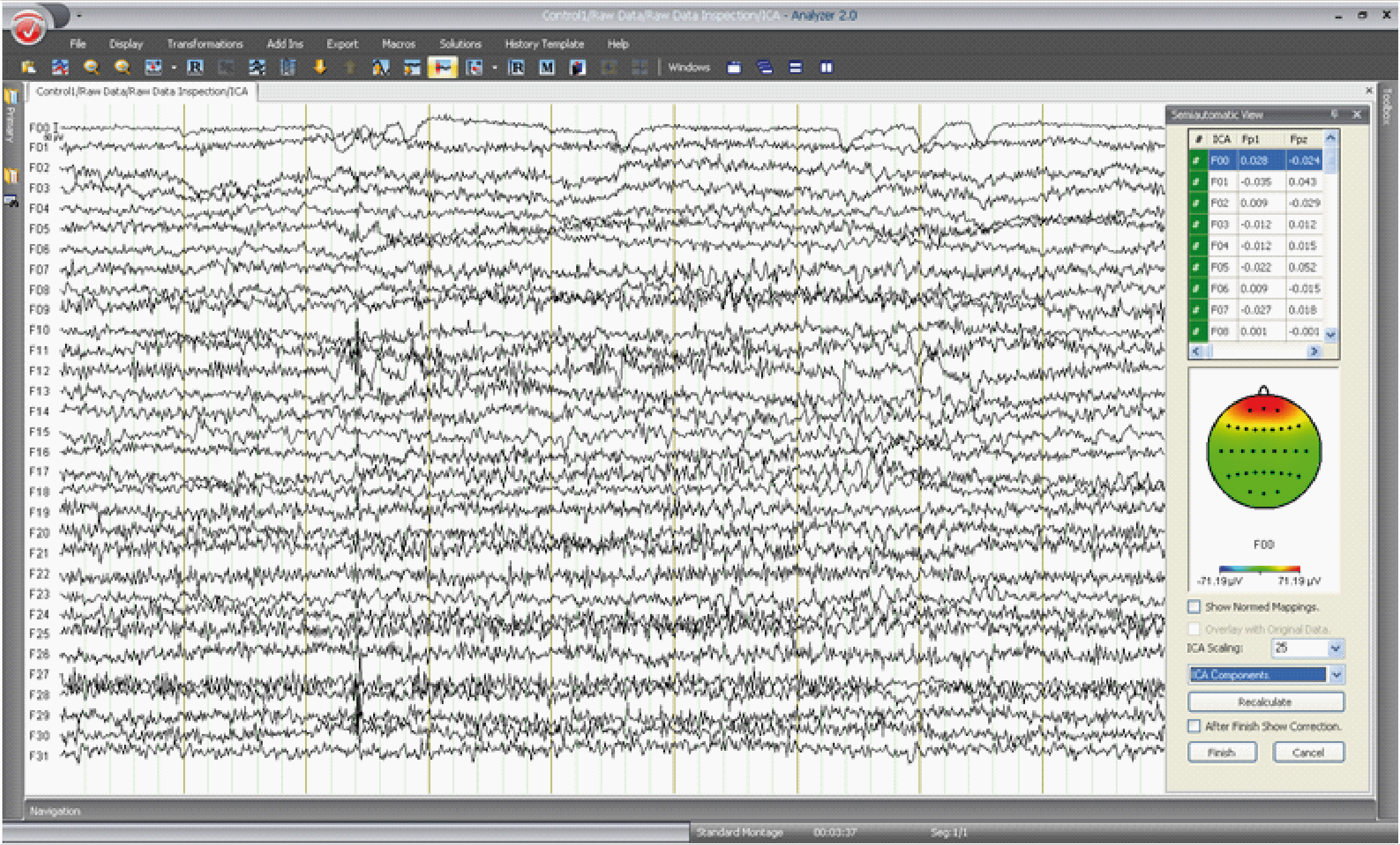
Figure 1
The first thing I would do is give your ICs some room. You have already read about how to do this in the last newsletter. And now, let’s have a play around!
So first I’ll describe the window – our playground. Then I’ll introduce some of the tools you can use and finally we’ll explore some ICs and see whether we can tell anything about them at a glance.
Ok, let’s start with the window. The first thing to catch the eye is the IC activity on the left side of the window but please take a look at the right hand side first. At the top you’ll see the list of your ICs. If you click on one of them it becomes blue and now at the bottom you’ll see the IC map. By the way, I know you probably expect to be able to customize the map just like any other map in Analyzer 2 and of course you’re right, you can do so the usual way (by Right-Click, choose Settings). If you double click on the green field in the first column it will turn red – I will tell you what this is for in a minute.
If you look a bit further down there is a drop-down menu which you see in Figure 2. The menu contains the following four items: ICA-Components, Correction, Subtracted and Topographies. These four views allow you to look at your ICs in a really exhaustive manner. So let’s spend some time on them.
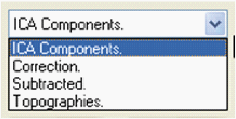
Figure 2
If you select ICA Components, the components are displayed first, as shown in Figure 1. Now you can use the transient view tool to find out the spectra of your ICs. Mark a time interval by right-clicking “FFT” from the transient views. You will get a frequency spectrum of the components. This is where Analyzer 2’s real power can be seen. Slide the marked interval over your data. The Analyzer 2 will continuously display the changing frequency spectra of the chosen time point as you slide over the data. By the way, if you have two screens on your computer you can even undock windows like the FFT-tool and drag it onto your second screen to have a better view of your data.
Do you want to see your corrected EEG with and without this or that suspicious component? If you select Correction, the reconstructed data set is displayed without the components highlighted in red. If you want to view the component in the corrected EEG or not, or see the EEG with or without a component – it is just a click away. But what was the original EEG like? Check “overlay with original data” and you will be shown how your data will change. Easy, right?
And what if I like viewing what information I’m going to remove from my data? If you select Subtracted, the reconstructed data set is displayed using only the components highlighted in red. See how the subtracted data changes depending on what components are checked or unchecked. Overlay this with the original EEG to see whether you’ve removed the correct information. Now do you understand why I talked about playing around?
Ok, there’s one more bit of important information that describes an IC. If you select topographies, the associated map view of all components is displayed. As you can’t really find a scaling factor to fit all maps I recommend displaying normalized maps (check the box in control panel). This view is very helpful to get a first general impression. This pattern of Figure 3’s third (F02) and fourth (F03) topography with their frontal and clear opposing activity make them candidates to contain the activity caused by horizontal eye movement.
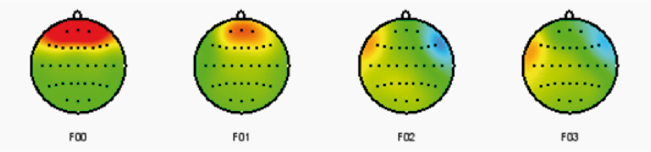
Figure 3
Because the ocular artifact is so prominent and with such distinct information – you are used to seeing it with your bare eyes – it can easily be identified by the ICA. Moreover, it is likely to be the first IC on your list of IC’s, as is the case in Figure 3. Analyzer 2.0 has a more sophisticated way of dealing with ocular artifacts, that is, ICA transform ocular correction. Though, the advantages and restrictions mentioned above are basically the same for this transform.
However, the simple approach of just looking at the ICs can lead to very good results. Figure 4 shows the corrected EEG overlaid with the original data (in red). What do you think – pretty good huh?

Figure 4
But we want to become experts, so let’s talk about some other, not so easy to spot artifacts.
Sometimes it just so happens that an electrode is prepared badly, or some electrodes may not function properly. I have heard that the latter does happen occasionally. Anyhow, the result of this will be that one of your channels contains mainly noise. Because this noise is not linked to any EEG information, the ICA will make a separate component out of this channel. A bad channel can easily be found on the ICA Maps. If you find a map with only one channel “active”, well, you guessed it. But watch out, if you look at a spline-interpolated map, a bad channel on the edge of the cap does look a bit like a component. Therefore it is sometimes helpful to use triangulation as interpolation to display the topographies.
Let’s come back to the experiment we used to discuss our subject. Possibly there is severe muscle activity in our data we can spot immediately. But what about data where we can’t see the artifact? Does this mean that there is none? Well, we should assume that the artifact is there. Now we can make things easier and filter it out, however, if cases where we are interested in higher frequencies, filtering is not an option. So, what can we do? Are you still with me, or are you already looking at the FFT of your ICs? After determining the ICs, which have high power in the higher frequency bands, you check their topographies. You are looking for components, with rather local activity on the edges of the cap. With an infra-cerebral-cap it’s often quite amazing. You can even connect the IC activity to a specific muscle. Moreover, the topography reflects the orientation of the electrical field the muscle produces.
ECG related artifacts
Ok, by now you’re almost an expert but let’s search for one more kind of artifact. You usually do not see any artifacts from the heart in your EEG. I’m afraid the bad news is that there is always some ECG related activity in your EEG. This time even the filter option won’t save you. So, how do you find an IC with ECG-activity? As the heart-related-activity has in many cases no clear topography you have to look at some other information. Let’s scale the IC activity so you see at least 20 seconds. This will make it easier to find activity with such a low frequency. And of course, look at the FFT transform of the ICs (to get a finer frequency resolution choose a wide interval (e.g. 4 second) to slide over the ICs). Is there an IC with a Peak in the range of 0.7 to 2 Hz?
I have to confess, that I do not always find this kind of activity. Clearly having more than 32 channels, let’s say 64 channels, helps a lot. I left this out when I discussed the theory of the ICA transform with you. However, the ICA assumes that there are more channels than sources. If this assumption is violated, the ICA has to mix the activity of some sources into one IC. The direct consequence is that you should record enough channels if you want to obtain really good results with the ICA transform.
By now we have looked at some ICs and we have seen how to identify some artifacts with a few clicks and by taking a quick look at them. Clearly this is not the only thing the ICA transform can do – in fact, that’s just the beginning. The Analyzer 2 provides you with all the information you need to calculate any kind of statistic on the components, or on the Matrices the ICA transform uses to calculate the ICs from the EEG and the EEG form the ICs.
Of course, I have not covered everything there is to know, however I hope you’ve now got enough enthusiasm to want to explore your data with the new Analyzer 2 ICA transform. And if you like working with it, I have some good news for you: We are enhancing the ICA transform even more. Stay tuned for a surprise…